Decoding Connectionist Temporal Classification
Being able to interpret the output probability matrix from the Convolutional Recurrent Neural Network (CRNN) is an essential task for getting output from the trained network. Various decoding techniques prove to be useful for this task. In this article, we’ll discuss two of those methods.
They are:
- Best Path Decoding
- Beam Search Decoding
In the following sections, we will first take a brief look at what Connectionist Temporal Classification (CTC) really is, and then explore both the decoding methods.
Revisiting CTC
Here is a short refresher on what Connectionist Temporal Classification (CTC) is.
CTC is a method using which we can train a Neural Network with the pair of images and ground truth texts without worrying about the width and position of the letter in the input image.
CTC works by encoding the text in a way that merges all the repeating chracters into a single character. For the repeating letters, CTC uses a pseudo-character denoted as “-“, in our examples. Fig.1 shows the output probability matrix from a CRNN. There are two time-steps and three characters (including one blank). At each time-step, the character score sums up to 1. Scores for all the possible alignments are added together for the corresponding ground truth for calculating the loss.
For a more detailed discussion readers are advised to go through “Explanation of Connectionist Temporal Classification”.
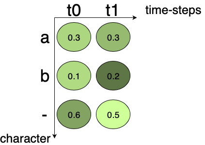
Fig.1 Output matrix from the Convolutional Recurrent Neural Network.
Best Path Decoding
Best path decoding is the easiest method for decoding the output probability matrix.
It works in the following manner:
- The first step entails calculating the best path by considering the character with the maximum probability at every time-step.
- The second step involves removing blanks and duplicate characters.
Let’s try to understand this by looking into an example. Fig.2 shows an output probability matrix from a CRNN. The character with the most probability for “t0” and “t1” are ‘-‘, and ‘-‘ respectively. Then decoding the text, we get the output as “”. We can calculate the probability for this path by multiplying the character probability as, 0.6x0.5 = 0.3 for this example.
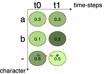
Fig.2 Best Path Decoding example, the dashed line in red shows the path with maximum character probability.
An advantage of this decoding technique is, it is very fast, as we only have to select the character with maximum probability at each time-step. If we have c characters and t time-steps, the algorithm has a run time of O(t.c).
But there are cases where this decoding technique fails.
Let us consider an example, if the ground truth is “a”, then all the possible paths for “a” are “aa”, “a-”, “-a“, as shown in Fig.3. But there are cases where this decoding technique fails. Summing up the score of the individual path we get, 0.09 + 0.15 + 0.18 = 0.42. As, 0.42 > 0.3 shows that “a” is more probable than “”. Hence, we need a better and efficient algorithm for taking care of such cases.
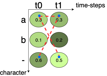
Fig.3 A case where Best Path Decoding fails. Here the dashed line in red shows the possible path for getting the letter “a”.
Beam Search Decoding
Beam search decoding is an algorithm which iteratively creates various individuals (equal to the size of the beam) and scores them. In this algorithm, beam-width is the only hyperparameter for getting better results. Beam-width decides the number of letters we wish to keep in the memory for checking various possibilities.
Let us consider our output probability matrix as an example of getting an intuitive feel of this algorithm. The matrix consists of alphabets {“a”, “b”} and blank character “-“, we will be considering the example with the beam-width equal to 2.
In Fig.4, you can see the tree for the output matrix shown in Fig.3. Here, we start with an empty beam “ “, which will act as the root node of the tree. We can take this beam and extend it to all the possible characters under consideration. We get one path for each beam with a probability of 0.3, 0.1, 0.6 for “a”, “b”, “-“ respectively. As we have beam-width equal to 2, we will not be considering “b” for the further expansion process. The process is again repeated for both the remaining beams.
This time the extended beams give us beam with a probability of 0.09, 0.06, 0.15, 0.18, 0.18, 0.3 for “aa”, “ab”, “a-“, “-a”, “-b”, “–” respectively. As these nodes will be our leaf nodes, we’ll merge the nodes with similar output. For example, we’ll merge “aa”, “a-“, and “-a” as they all are equal to “a”. After doing this we are left with 3 beams with probability of 0.42, 0.18, 0.3 for “a”, “-b”, “–” respectively. We get rid of “-b” as we have a beam-size of 2 and it has the lowest probability. Now, it is clear that, by using the beam search decoding algorithm we were able to reach the correct solution, which is “a”.
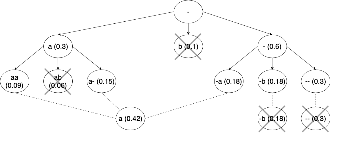
Fig.4 Beam Search Decoding visualised as a tree with “a”, “b” and beam-width as 2. Number in the bracket is the probability for that character, solid lines show new beams and dotted lines shows merging of similar characters
Here is an implementation for this algorithm:
def beam_search_decoder(probability_matrix, beam_width):
    """
    This method is used to get the most probable candidates using beam search decoding algorithm
    probability_matrix: A numpy array of shape (batch_size, number_of_classes)
    beam_width: int denoting beam size
    """
    sequences = [[list(), 1.0]]     # Initializing an empty list for storing sequences and scores
    # iterating through all the steps in the sequence
    for row in probability_matrix:
        all_candidates = list()
        # expand each current candidate
        for i in range(len(sequences)):
            seq, score = sequences[i]   # Getting score and individual sequence
            for j in range(len(row)):
                # getting score for indiviual class (character)
                candidate = [seq + [j], (score * row[j])]
                all_candidates.append(candidate)
        # arrange all candidates by score
        ordered = sorted(all_candidates, key=lambda tup:tup[1], reverse=True)
        # select the best candidates
        sequences = ordered[:beam_width]
    return sequences
In this code, we begin with a list of empty sequences which will contain candidate beams with the corresponding score. Then we loop through the probability matrix. In this loop, we get the previous best sequence and then expand them by looping through all the classes (characters). In this manner, we get a list of possible sequences with scores which is further sorted and we get beams equal to the beam-width.
Advantage of using this decoding method is that it explores a larger number of solutions. But, it is slow when compared to the best path decoding algorithm. If we have c characters, t time-steps and k beam_width, the algorithm has a run time of O(c.t.k).
Conclusion
In this article, we saw two different methods of decoding the output probability matrix from a Convolutional Recurrent Neural Network trained using Connectionist Temporal Classification. Both methods have their pros and cons. It is necessary to analyse the use-case and use the algorithm best suited for that case.